Most unsupervised learning algorithms attempt to learn all that there is to know about the environment, with no selectivity. They flail about, often at random, attempting to learn every possible fact. It takes them far too long to learn a mass of mostly-irrelevant data. For example, [Drescher 91] introduces an algorithm for building successively more powerful descriptions of the results of taking particular actions in an unpredictable world. However, his algorithm scales poorly, and hence is unsuitable for realistic worlds with many facts, given the current state of computational hardware. Since its running speed decreases as more is learned about the world, the algorithm eventually becomes unusably slow, just as the agent is learning enough to make otherwise useful decisions.
A real creature does not do this. Instead, it uses different focus of attention mechanisms, among others perceptual selectivity and cognitive selectivity, to guide its learning. By focusing its attention to the important aspects of its current experience and memory, a real creature dramatically decreases the perceptual and cognitive load of learning about its environment and making decisions about what to do next. This research uses the same methods to build a computationally tractable, unsupervised learning system that might be suitable for use in a autonomous agent that must learn and function in some complex world.
This paper presents an algorithm for learning statistical action models which incorporates perceptual and cognitive selectivity. In particular, we implemented a variation on Drescher's schema mechanism and demonstrate that the computational complexity of the algorithm is significantly improved without harming the correctness of the action models learned. The particular forms of perceptual and cognitive selectivity that are employed represent domain-independent heuristics for focusing attention that potentially can be incorporated into any learning algorithm.
The paper is organized as follows. Section 2 discusses different notions of focus of attention, and in particular focused on heuristics for perceptual and cognitive selectivity. Section 3 describes the algorithm implemented and the microworld used. Section 4 elaborates on the experimental results obtained. Section 5 lists some shortcomings and discusses future extensions. Finally, section 6 discusses related work.
Along another dimension, there is a distinction between domain-dependent and domain-independent methods for focus of attention. Domain-independent methods represent general heuristics for focus of attention that can be employed in any domain. An example is to only attempt to correlate events that happened close to one another in time. Domain-dependent heuristics, on the other hand, are specific to the domain at hand. They typically have been preprogrammed (by natural or artificial selection or by a programmer). For example, experiments have shown that when a rat becomes sick to its stomach, it will assume that whatever it ate recently is causally related to the sickness. That is, it is very hard for a rat to learn that a light flash or the sound of a bell is correlated to the stomach problem because it will focus on recently eaten food as the cause of the problem [Garcia 72]. This demonstrates that animals have evolved to pay attention to particular events when learning about certain effects.
Finally, the focus mechanism can be goal-driven and/or world-driven. Focus of attention in animals is both strongly world- and goal-dependent. The structure of the world determines which sensory or memory bits may be "usually" ignored (e.g. those not local in time and space), while the task determines those which are relevant some of the time and not at other times. For example, when hungry, any form of food is a very important stimulus to attend to.
The results reported in this paper concern world-dependent, but goal-independent, as well as domain-independent cognitive and sensory selectivity. Such pruning depends on constant properties of the environment and common tasks, and does not take into account what the current goal of the agent is. The methods can be applied to virtually any domain. While it is true that, in complex worlds, goal-driven and domain-dependent pruning is quite important, it is surprising how much of an advantage even goal-independent pruning can convey. Goal-driven and domain-dependent strategies for focus of attention are briefly discussed in the future research section.
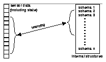
Obvious physical dimensions along which to be perceptually selective include spatial and temporal selectivity. The universe tends to be spatially coherent: causes are generally located nearby to their effects (for example, pushing an object requires one to be in contact with it). Further, many causes lead to an observable effect within a short time (letting go of an object in a gravity field causes it to start falling immediately, rather than a week later). Real creatures use these sorts of spatial and temporal locality all the time, often by using eyes that only have high resolution in a small part of their visual field, and only noticing correlations between events that take place reasonably close together in time. While it is certainly possible to conceive of an agent that tracks every single visual event in the sphere around it, all at the same time, and which can remember pairs of events separated by arbitrary amounts of time without knowing a priori that the events might be related, the computational burden in doing so is essentially unbounded.(1) The algorithm discussed in section 3 implements temporal selectivity as well as spatial selectivity to reduce the number of sensor data that the agent has to correlate with its internal structures (see the figure above). Note that the perceptual selectivity implemented is of a "passive" nature: the agent prunes its "bag of sensory bits," rather than changing the mapping of that bag of bits to the physical world by performing an action that changes the sensory data (such as changing its point of view).The latter would constitute active perceptual attention).
Notice that for any agent that learns many facts, being cognitively selective is likely to be even more important than being perceptually selective, in the long run. The reasons for this are straightforward. First, consider the ratio of sensory to memory items. While the total number of possible sensory bits is limited, the number of internal structures may grow without bound. This means that, were we to use a strategy which prunes all sensory information and all cognitive information each to some constant fraction of their original, unpruned case, we would cut the total computation required by some constant factor---but this factor would be much larger in the cognitive case, because the number of facts stored would likely far outnumber the number of sensory bits available.
Second, consider a strategy in which a constant number of sensory bits or a constant number of remembered facts are attended to at any given time. This is analogous to the situation in which a real organism has hard performance limits along both perceptual and cognitive axes; no matter how many facts it knows, it can only keep a fixed number of them in working memory. In this case, as the internal structures grow, the organism can do its sensory-to-memory correlations in essentially constant time, rather than the aforementioned O(n2) time, though at a cost: as its knowledge grows, it is ignoring at any given time an increasingly large percentage of all the knowledge it has.
Compromise strategies which keep growth in the work required to perform these correlations within bounds (e.g., less than O(n2)), yet not give in completely to utilizing ever-smaller fractions of current knowledge (e.g., more than O(1)) are possible. One way to compromise is to use the current goal to help select what facts are relevant; such goal-driven pruning will be discussed later. Since generally only a small number of goals are likely to be relevant or applicable at any one time (often only one), this can help to keep the amount of correlation work in bounds.(2)
Similarly, one can use the world or sensor data to restrict the number of structures looked at (as is the case in the algorithm described in this paper). Not all internal structures are equally relevant at any given instant. In particular, internal structures that refer neither to current nor expected future perceptual inputs are less likely to be useful than internal structures which do. This is the particular domain-independent, goal-independent, world-driven heuristic for cognitive selectivity which is employed in the algorithm described in the next section. Again, in real creatures domain-dependent and goal-driven cognitive selectivity play a large role too. For example, the subset of internal structures that are considered at some point in time is not only determined by what the agent senses and what it expects to sense next, but also by what it is "aiming" to sense or not sense (i.e., the desired goals). Goal-driven and domain-dependent solutions to cognitive selectivity are discussed in the future research section.
Drescher is interested in Piagetian modeling, so his microworld is oriented towards the world as perceived by a very young infant (less than around five months old). The simplified microworld (which is shown below) consists of a simulated, two-dimensional "universe" of 49 grid squares (7 by 7). Each square can be either empty or contain some object. Superimposed upon this universe is a simulated "eye" which can see a square region 5 grid squares on a side, and which can be moved around within the limits of the "universe". This eye has a "fovea" of a few squares in the center, which can see additional details in objects (these extra details can be used to differentiate objects enough to determine their identities). The universe also consists of a "hand" which occupies a grid square, and can bump into and grasp objects. (The infant's arm is not represented; just the hand.) An immobile "body" occupies another grid square.
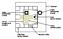
Every sensory item is represented in the simulation as a single bit. In Drescher's original algorithm, there is no grouping of these bits in any particular way (e.g., as a retinotopic map, or into particular modalities); the learning algorithm sees only an undifferentiated "bag of bits".
The "facts" learned by this system are what Drescher calls schemas. They consist of a triple of context (the initial state of the world, as perceived by the sensory system), the action taken on this iteration, and result (the subsequent perceived state), which maps actions taken in a particular configuration of sensory inputs into the new sensory inputs resulting from that action. A typical schema might therefore be, "If my eye's proprioceptive feedback indicates that it is in position (2,3) [context], and I move my eye one unit to the right [action], then my eye's proprioceptive feedback indicates that it is in position (3,3) [result]." Another typical schema might be, "If my hand's proprioceptive feedback indicates that it is in position (3,4) [context], and I move it one unit back [action], I will feel a touch on my mouth and on my hand [result]" (this is because the hand will move from immediately in front of the mouth to in contact with the mouth). Notice that this latter schema is multimodal in that it relates a proprioceptive to a tactile sense; the learning mechanism and its microworld build many multimodal schema, relating touch to vision, vision to proprioception, taste to touch (on the mouth), graspability to the presence of an object near the hand, and so forth. It also creates unimodal schemas of the form illustrated in the first schema above, which relates proprioception to proprioception.
A schema is deemed to be reliable if its predictions of context, action, result are accurate more than a certain threshold of the time. A schema maintains an extended context and an extended result which keep statistics for every item not yet present in the context or result so as to detect candidates for spinning off a new schema. If we already have a reliable schema, and adding some additional sensory item to the items already expressed in either its context or its result makes a schema which appears that it, too, might be reliable, we spin off a new schema expressing this new conjunction. Spinoff schemas satisfy several other constraints, such as not ever duplicating an existing schema, and may serve to be the basis for additional spinoffs themselves later.
The behavior of the world is allowed to be nondeterministic (e.g., actions may sometimes fail, or sensory inputs may change in manners uncorrelated with the actions being taken), and each schema also records statistical information which is used to determine whether the schema accurately reflects a regularity in the operation of the world, or whether an initial "guess" at the behavior of the world later turned out to be a coincidence.(4)
The possible sensory inputs consist of all bits arriving from the "eye", proprioceptive inputs from eye and hand (which indicate where, relative to the body, the eye is pointing or the hand is reaching), tactile inputs from the hand, and taste inputs from the mouth (if an object was in contact with it). The "eye" reports only whether an object (not which object, only the presence of one) is in a grid square or not, except in its central fovea, where it reports a few additional bits if an object was present. The "infant" does not have a panoramic knowledge of all 49 squares of the universe at once; at any given instant, it only knows about what the eye can see, what the hand is touching, or what the mouth is tasting, combined with proprioceptive inputs for eye and hand position. In particular, certain senses, viewed unimodally, are subject to perceptual aliasing [Whitehead and Ballard 90]: for example, if a schema mentions only a particular bit in the visual field, without also referring to the visual proprioceptive inputs (which determine where the eye is pointing), then that schema may be subject to such aliasing. Similarly, any schema mentioning any visual-field sensory item that is not in the fovea may alias different objects, since the non-foveal visual field reports only the presence or absence of an object in each position, rather than the exact identity of the object in question. In Drescher's original implementation, the system spent most of its time (a fixed 90%) taking random actions and observing the results. The remaining 10% of its time was spent taking actions which had led to some reliable outcome before, to see if actions could be combined.(5)
 ), for which schema numbers (
 ). Second, we must decide whether to spin off a new schema; this is the "learning" part of the algorithm, and here the focus mechanism dictates which item numbers to check for reliability (
 ) for which schema numbers (
 ). Thus, our choice of these four sets of numbers determines which sensory items and schemas are used in either updating our perception of the world, or deciding when a correlation has been learned. Stati and Stats determine the perceptual selectivity, while Spini and Spins determine the cognitive selectivity.
------------------------------------
                Statistics  Spinoffs
------------------------------------
Which items?    (fig)       (fig)
Which schemas?  (fig)       (fig)
------------------------------------
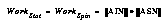
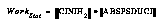
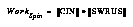
The algorithm does the vast majority of its work in two inner loops (one for updating statistics, reflecting what is currently perceived, and one for deciding whether to spin off new schemas, reflecting learning from that perception). The number of items or schemas selected at any given clock tick determines the amount of work done by the learning algorithm in that tick. Thus, if  is the work done during the statistical-update part of the algorithm (e.g., perceiving the world) of any one clock tick, and
  is similarly the amount of work done in deciding which spinoff schemas to create, then the work done during either one is the product of the number of items attended to and the number of schemas attended to, or:
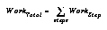
Thus, the behavior of WorkStep over time tells us how well the algorithm will do at keeping up with the real work, e.g., how fast it slows down as the number of iterations, hence schemas, increases.
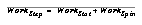
A way of evaluating the utility of various algorithms is to examine the amount of work performed per schema (either reliable schemas or all schemas; the former being perhaps the more useful metric):
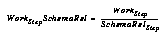
which is simply the amount of work performed during some steps divided by the number of reliable schemas generated by that work.(6) A similar definition for total schemas over total work is straightforward.(7)
An algorithm which determines these choices is thus described by the pairs << ,
, >,<
>,< ,
, >>; we will call each element a selector.
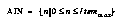
A little more terminology will enable us to discuss the actual selectors used.  is the number of schemas currently learned.
  is the number of sensory items.
  is the value of sensory bit n, and
  is the value of that item at some time t.
  denotes some schema s which is dependent upon (e.g., references in its context or result) some item i.
and Stats and Spins use the selector all schema numbers, or ASN:
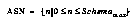
This means that the basic algorithm does a tremendous amount of work in the two n x m inner loops, where n is the size of the set of items in use,  , and similarly m is the size of the set of schemas in use,
  . Hence,
It can eventually learn a large number of facts about the world in this way, but it runs slowly, and becomes increasingly slow as the number of known facts increases.
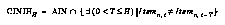
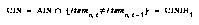
while Spini used a specialization of this, in which the history is only the very last event, which we shall call the changed item numbers, or CIN, selector for compactness:
Similarly, the schemas used were as follows. Consider the set all bare schemas, or ABS, which consists only of schemas which make no predictions about anything (there is one of these per action at the start of any run, and no other schemas; this is the root set from which new schemas which predict correlations between actions and sensory inputs may be spun off):
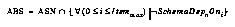
To define Stats, we add to these schemas dependent upon changed items, to get:

This selector is a special case of the more general one (which uses an arbitrary-length history), in that it uses a history of length 1. The general case, of course, is:
Finally, Spins is defined as schemas with recently updated statistics, or
Adding these changes amounts to adding some simple lookup tables to the basic algorithm that track which items were updated in the last clock tick, and, for each item, which schemas refer to it in their contexts or results, then using these tables to determine which sensory items or schemas will be participants in the statistical update or spinoffs. Such tables require a negligible, constant overhead on the basic algorithm.
The perceptual and cognitive strategies above place a high value on novel stimuli. Causes which precede their effects by more than a couple of clock ticks are not attended to. In the world described above, this is perfectly reasonable behavior. If the world had behaviors in it where more prior history was important, it would be necessary to attend further back in time to make schemas which accurately predicted the effects of actions.
These particular strategies also place a high value on a very specific spatial locality. Even sensory items that are very near items which have changed are not attended to. Since this microworld only has objects which are one bit wide, and the actions which involve them are, e.g., touch (which requires contact), this is the right strategy. (8)
The computational complexity of the two n x m inner loops is reduced by these selectors as follows:
In any run which generates more than a trivial number of schemas or has more than a handful of sensory bits, this is a dramatic reduction in the complexity, as shown in the table on page 8.
Another manual method of checking the results employed n-way comparisons of the generated schemas themselves. The (context, action, result) triple of each schema can be represented relatively compactly in text (ignoring all the statistical machinery that also makes up a schema); by sorting the schemas generated in any particular run into a canonical order, and then comparing several runs side-by-side, one can gain an approximate idea of how different runs fared. The figure at the top of this page demonstrates a tiny chunk from a 5-way comparison of a certain set of runs, in which 5 somewhat-different runs were compared for any large, overall changes to the types of schemas generated.
A simple way to establish what the agent knows is therefore to use the generated schemas as parts of a plan, "chaining" them together such that the result of one schema serves as the context of the next, and to build these chains of schemas until at least one chain reaches from the initial state of the microworld to the goal state. If we can build at least one such chain, we can claim that the agent "knows" how to accomplish the goal in that context; the shortness of the chain can be used as a metric as to "how well" the agent knows.(9) For this task, the schemas to be used should be those deemed "reliable", e.g., those which have been true sufficiently often in the past that their predictions have a good chance of being correct. Simply employing all schemas, reliable or not, will lead to many grossly incorrect chains.
At the start, no facts about the world are known, hence no chain of any length can be built. However, after a few thousand schemas are built (generally between 1000 and 5000), most starting states can plausibly chain to a simple goal state, such as centering the visual field over the hand, in a close-to-optimal number of steps.
Given this mechanism, how well did the focus of attention mechanisms fare? Quite well. In general, given the same approximate number of generated schemas, both the basic and focused approaches cited above learned "the same" information: they could both have plausibly short chains generated that led from initial states to goals. Both the chaining mechanism described above, and manual inspection, showed no egregious gaps in the knowledge or particular classes or types of facts that failed to be learned.
As shown in the figure on the next page, the focused approach tended to require approximately twice as many timesteps to yield the same number of schemas as the unfocused approach. This means that a real robot which employed these methods would require twice as many experiments or twice as much time trundling about in the world to learn the same facts. However, the reduction of the amount of computation required to learn these facts by between one and two orders of magnitude means that the processor such a robot must employ could be much smaller and cheaper---which would probably make the difference between having it onboard and not. This is even more compelling when one realizes that these computational savings get bigger and bigger as the robot learns more facts.
Because of this, the only way that any learning algorithm which uses this system could learn "incorrect" facts (e.g., correlations that do not, in fact, reflect true correlations in the world) would be to systematically exclude relevant evidence that indicates that a schema that is thought to be reliable is in fact unreliable. No evidence of this was found in spot checks of any test runs. It is believed (but not proved) that none of the algorithms here can lead to such systematic exclusion of relevant information: the mechanism may miss correct correlations (such is the tradeoff of having a focus of attention in the first place), but it will not miss only the correlations that would tend to otherwise invalidate a schema thought to be reliable.
The results in this table were all produced by runs 5000 iterations long. Similar runs of two or three times as long have produced comparable results.
The first four columns of the table show the particular selectors in use for any given run; the top row shows those selectors which correspond to the basic (Drescher) algorithm, while the bottom row shows the most highly-focused algorithm, as described in section 3.4 above.
The table is sorted in order by its last column, which shows number of reliable schemas generated during the entire 5000-iteration run, divided by the amount of total work required. For conciseness, we shall call the value in this column  , which is defined as:
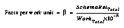
where the multiplication by 10-6 is simply to normalize the resulting numbers to be near unity, given the millionfold ratio between work units and number of schemas generated.
The bold rows in the table show successive changes to the selectors used, one at a time. The top row is the basic algorithm, which shows that about a billion total inner loops were required to learn 1756 schemas, 993 of which were reliable, which gives a  of 0.9.
Let us examine changes to the selectors for spinoffs, which determine the cognitive selectivity, or what is attended to in learning new schemas from the existing schemas. When we change Spini from AIN to CIN, the amount of work drops by about a factor of two, while the number of generated schemas barely decreases. This means that virtually all schemas made predictions about items which changed in the immediately preceeding clock tick (e.g., that corresponding to the action just taken), hence looking any further back in time for them costs us computation without a concomittant increase in utility.
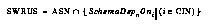
Changing Spins from ASN to SWRUS, given that Spini is already using the selector CIN, yields a small improvement in  (not visible at the precision in the table), and also a small improvement in the ratio of reliable to total schemas. (Were Spini not already CIN, the improvement would be far more dramatic, as demonstrated in runs not shown in the table.) Note, however, the enormous decrease in the amount of work done by the spinoff mechanism when Spins changes from ASN to SWRUS, dropping from 10% of WorkTotal to 1%.
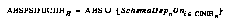
Next, let us examine the effects of perceptual selectivity. Changing Stats from ASN to ABSPSDUCI increases  by a factor of 5.4, to 9.2, by decreasing the amount of work required to update the perceptual statistics by almost an order of magnitude. In essence, we are now only bothering to update the statistical information in the extended context or extended result of a schema, for some particular sensory item in some particular schema, if the schema depends upon that sensory item.
Various selectors versus number of schemas and total
                     computation, for 5000 iterations.
------------------------------------------------------------------------------------------------------------------------------------------------------
Items              Schemas    Items                Schema     Total     Rel   T/R   Spin                Stat  Both  Spin                   Stats  Both
------------------------------------------------------------------------------------------------------------------------------------------------------
AIN                ASN        AIN                  ASN        1756      993   1.77  533                 533   1066  1.9                    1.9    0.9
AIN                ASN        CINIH                ABSPSDUCI  1135      403   2.82  398                 12    410   1.0                    33.6   1.0
AIN                ASN        AIN                  ASN        1794      1075  1.67  533                 532   1065  2.0                    2.0    1.0
AIN                ASN        AIN                  ABSPSDUCI  1110      518   2.14  391                 55    446   1.3                    9.4    1.2
CIN                ASN        AIN                  ASN        1693      948   1.79  44                  524   568   21.5                   1.8    1.7
CIN                SWRUS      AIN                  ASN        1395      791   1.76  2                   463   466   316.4                  1.7    1.7
CIN                ABSPSDUCI  AIN                  ASN        1622      924   1.76  15                  510   525   61.6                   1.8    1.8
CIN                ASN        AIN                  ABSPSDUCI  1110      506   2.19  33                  54    87    15.3                   9.4    5.8
CIN                ABSPSDUCI  AIN                  ABSPSDUCI  1110      506   2.19  10                  54    64    50.6                   9.4    7.9
CIN                ABSPSDUCI  CINIH                ASN        1366      643   2.12  13                  64    77    49.5                   10.0   8.4
CIN                ASN        CINIH                ABSPSDUCI  1136      399   2.85  34                  12    46    11.7                   33.3   8.7
CIN                SWRUS      AIN                  ABSPSDUCI  1102      498   2.21  1                   53    54    415.0                  9.4    9.2
CIN                SWRUS      CINIH                ASN        1353      688   1.97  2                   64    66    275.2                  10.8   10.3
CIN                ABSPSDUCI  CINIH                ABSPSDUCI  1136      399   2.85  10                  12    22    40.7                   33.3   18.3
CIN                SWRUS      CINIH                ABSPSDUCI  1134      398   2.85  1                   12    13    331.7                  33.2   30.2

------------------------------------------------------------------------------------------------------------------------------------------------------
Finally, examine the last bold row, in which Stati was changed from AIN to CINIH.  increases by a factor of 3.2, relative to the previous case, as the amount of statistical-update work dropped by about a factor of four. We are now perceiving effectively only those changes in sensory items which might have some bearing in spinning off a schema which already references them.
Note that each successive tightening of the focus has some cost in the number of schemas learned in a given number of iterations. This means that, e.g., a real robot would require increasingly large numbers of experiments in the real world to learn the same facts. However, this is not a serious problem, since, given the focus algorithm described here, such a robot would require only about twice as many experiments, for any size run, as it would in the unfocused algorithm. This means that its learning rate has been slowed down by a small, roughly constant factor, while the computation required to do the learning has dropped enormously.
[Kaelbling and Chapman 90] propose a technique (the G algorithm) for using statistical measures to recursively subdivide the world known by an agent into finer and finer pieces, as needed, making particular types of otherwise intractable unsupervised learning algorithms more tractable. One could view that as an example of perceptual selectivity: the agent gradually increases the set of state variables that are considered, as needed, when selecting actions and learning (updating statistics).
[Chapman 90] describes a system that uses selective visual attention to play a video game. Even though the principles described are general, the particular methods used by his agent are very domain-dependent (they are specific to the particular problems his agent faces). Chapman is less concerned with how focus of attention and learning correlate. Instead he focuses on how to reduce the problem of perception and the inferencing problem by the use of visual routines.
Finally, all classifier systems have a built-in mechanism for generalizing over situations as well as actions and thereby perform some form of selective attention. In particular, a classifier may include multiple "don't care" symbols which will match several specific sensor data vectors and actions. This makes it possible for classifier systems to sample parts of the state space at different levels of abstraction and as such to find the most abstract representation (or the set of items which are relevant) of a classifier that is useful for a particular problem the agent has. [Wilson 85] argues that the classifier system does indeed tend to evolve more general classifiers which "neglect" whatever inputs are irrelevant.